Learning to Remember (and Forget)
The Evolution of Memory in Neural Networks
Recurrent Neural Networks
A major limitation of vanilla neural networks is that they are unable to process variable-length structures: they map fixed-length inputs to fixed-length outputs by learning features over a fixed number of layers. Further, traditional neural networks have no “memory”—when presented with sequential data such as this sentence, there is no easy way to use context learned from previous inputs to inform future outputs.
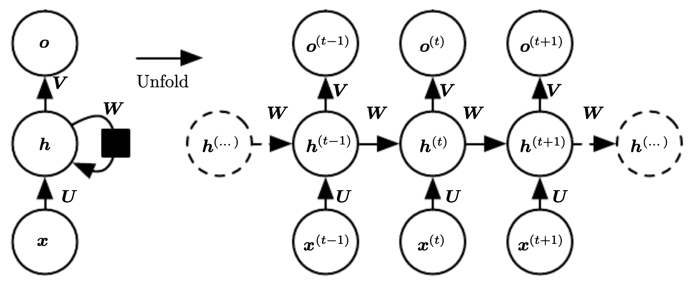
Unrolling a sequence-to-sequence RNN (Deep Learning. Goodfellow et al., 2016).
Recurrent neural networks (RNNs) are a class of neural networks specialized for sequential data. They can learn dependencies from previous inputs in the sequence though a self-loop connection which maintains a hidden state. As a result, RNNs also have the advantage of sharing the same parameters over time steps, much like a 1D temporal convolution. At each time step $t$, the network updates the hidden state $h_t$ using the learned parameters $\theta$, the previous hidden state $h_{t-1}$, and an input $x_t$ if applicable. The hidden step at each time step can be written $h_t = f(h_{t-1},,x_t;, \theta_h)$, where $f$ is the transformation of the hidden layer. The hidden state effectively encodes a limited summary of relevant features from all previous input sequence vectors. The output can be written $o_t = g(h_{t};, \theta_t)$, where $g$ is the transformation of the output layer.
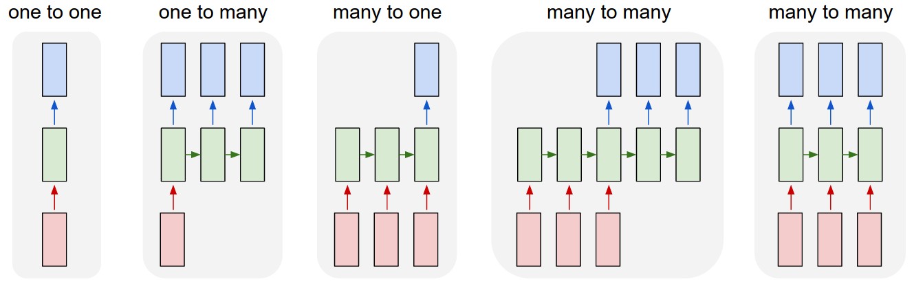
Various basic RNN architectures (Karpathy, 2015).
A helpful way to visualize RNNs is to unroll them into a chain of repeated feedforward networks that share the same parameters at each timestep. There are several basic RNN structures including one-to-one, one-to-many, many-to-one, and many-to-many. Each is used for different applications. For example, one-to-one would be appropriate for vanilla neural network tasks such as image classification. Unsynced many-to-many could be used for translation tasks, taking in a sentence in one language and producing a corresponding sentence in the target language, while synced many-to-many could be used for frame-by-frame video classification (Karpathy, 2015).
Using the unrolled view of the RNN, we can use backpropagation to learn the model parameters just as we do with feedforward networks. Since this backpropagation is performed over the states at different time steps, the algorithm is called backpropagation through time (BPTT).
A well-known problem with RNNs is that they struggle to capture long-term dependencies, or remembering information over longer sequences. Consider the following sentence:
“The dog, which was a golden retriever with a friendly disposition and a penchant for chasing squirrels in the park near the old oak tree where children often played on sunny afternoons, wagged its tail.”
There is a long-term dependency between “The dog” at the beginning of the sentence and “wagged its tail” near the end. A model trying to predict that “wagged its tail” comes after dependent clause in the middle of the sentence must keep “dog” as the subject of the sentence despite all of the added context. Since there is a large distance between the two relevant phrases, the gradients calculated by BPTT will tend to vanish (or, less commonly, explode) as a result of repeated matrix multiplication, and the model will not be able to learn their connection.
Long Short-Term Memory
To address the vanishing/exploding gradients problem, Long Short-Term Memory (LSTMs) were proposed. LSTMs are a type of gated RNN that are able to learn long-term dependencies. Individual LSTM cells replace the hidden state of the RNN with a more complicated recurrent network that includes an additional linear self-loop, allowing gradients to flow over long periods, subject to gating units. These gating units are dependent on the previous cell’s state as well as the input sequence, allowing the LSTM to dynamically forget or add new information depending on context.
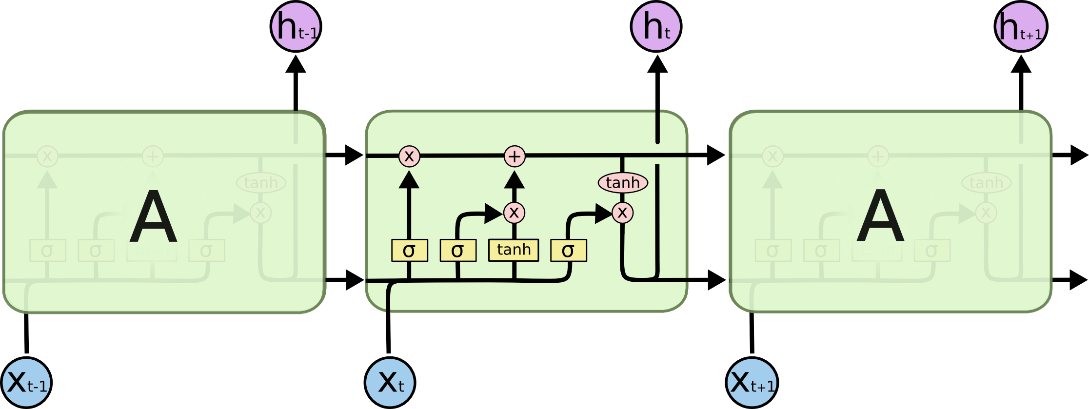
The inner workings of a LSTM cell (Olah, 2015).
The first gate is the forget gate, which weights the input vector and previous cell state and applies a sigmoid layer to squash the values between 0 and 1. The resulting vector is multiplied pointwise to the current cell state. This gate decides how much of the old information should be thrown out, with 0 representing deleting everything and 1 representing keeping everything. The next gate is the input gate, which decides how much and which new information is let in. A tanh and sigmoid layers are separately applied to the input to normalize the vector and determine each new feature input’s importance, respectively. The two resulting vectors are multiplied together pointwise before being added to the cell state. Finally, the cell state is put through a tanh layer before being multiplied with the output gate sigmoid, controlling what information is returned and passed to the next cell state.
There are other versions of the LSTM cell such as the Gated Recurrent Unit (GRU), which have different variations of the gating mechanism.
From Sequence-to-Sequence to Attention
Another pitfall of vanilla neural networks is that they are unable to process variable-length structures: they map fixed-length inputs to fixed-length outputs by learning features over a fixed number of layers. RNNs can be be extended to mapping between variable-length sequences, allowing them to handle complex tasks such as machine translation and speech recognition.
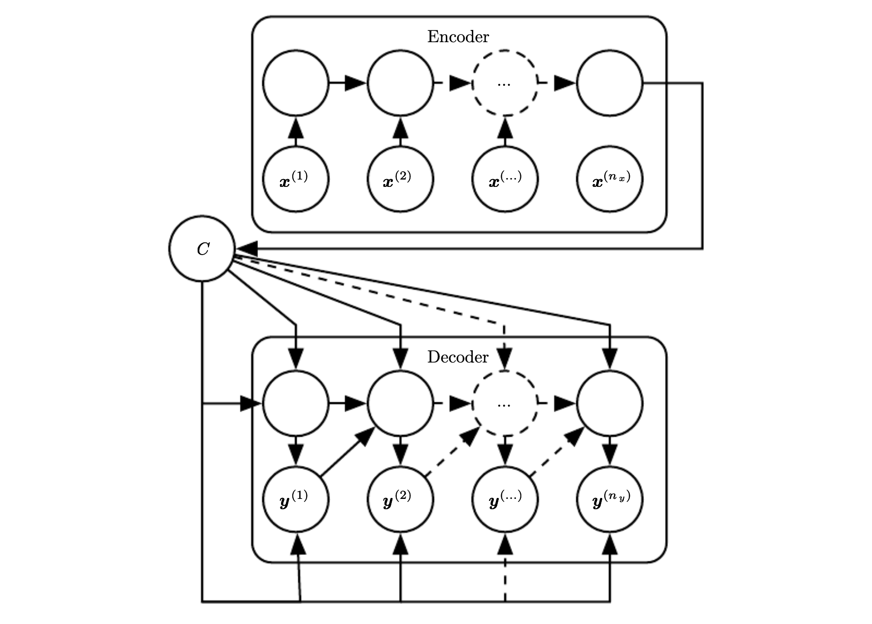
Sequence-to-sequence encoder-decoder architecture (Deep Learning. Goodfellow et al., 2016).
The sequence-to-sequence model proposed by Cho et al., 2014 and Sustekever et al., 2014 achieves this by using an encoder-decoder architecture. It reads the input sequence and encodes a fixed-length context vector $C$, which is then taken as input to a decoder that generates an output sequence. Here, the encoder and decoder are both RNNs composed of LSTM cells or a similar gated network.
This formulation, however, is once again limited by the requirement that $C$ must be of fixed length. For a longer sequences, the context vector would have a hard time encoding a good representation of all of the information.
To address this issue, Bahdanau, et al., 2016 introduced the attention mechanism. Instead of generating the output from a single fixed context vector, the decoder calculates a different context vector using all of the for each output word by weighting each hidden state of the encoder by an alignment score.
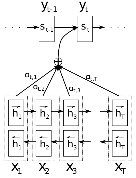
RNN-based attention model (Bahdanau, et al., 2016).
Suppose that we have input sequence $\textbf{x} = [x_1,\dots,x_{T_x}]$ of length $T_x$ and target sequence $\textbf{y} = [y_1,\dots,y_{T_y}]$ of length $T_y$. The encoder, implemented as a bidirectional RNN to try to capture the context of words both before and after the target word, has hidden states $\textbf{h} = [h_1,\dots,h_{T_x}]$. The context vector $c_i$ for each target word $y_i$ is calculated as a weighted sum of all of the hidden states: $$ \begin{aligned} c_i = \displaystyle\sum_{j=1}^{T_x}\alpha_{ij}h_j \end{aligned} $$ The weights $a_{ij}$ are the alignment scores given by: $$ \begin{aligned} \alpha_{ij} = \frac{\exp(a(s_{i-1},h_j))}{\Sigma_{k=1}^{T_x}\exp(a(s_{i-1},h_k))} \end{aligned} $$ where the alignment model $a$ is a feedforward neural network that predicts the relevance of the inputs at position $j$ to the output at position $i$.